Efficient AI

Quantization Basics

Aditya Desai

What is quantization?

Quantization maps a continuous (or large) set of values to a smaller discrete set.

There are two maps to keep track of:

  • The quantization map sends a real value to a code: \[ Q: X \rightarrow \{0,\dots,|Y|-1\} \]
  • The dequantization map reconstructs an approximate real value from that code: \[ Q^{-1}: \{0,\dots,|Y|-1\} \rightarrow \mathbb{R} \]
Reconstruction error

If the only goal is to store and recover data, then a natural metric is reconstruction error.

For values drawn from a distribution $P$, this is the mean squared error:

\[ \mathrm{Quantization\ error} = \mathbb{E}_{x\sim P} \bigl[ \| x - Q^{-1}(Q(x)) \|_2^2 \bigr]. \]

When reconstruction is not enough

Q. Should we always care about reconstruction loss?

A. No — it depends on how the quantized data is used.

For example, if we quantize weights $W$, we may care more about the downstream loss or about inner products than about $\|W-\hat W\|_2$.

This distinction is important in ML: a quantizer that looks good by reconstruction error may not be the one that preserves model quality.

How computers represent numbers

Computers already quantize numbers: a dtype determines which values are representable.

Before designing our own low-bit maps, recall the two basic families of number formats.

Integer formats

(A) Integer formats

Example: signed INT32.

  • Max: $2^{31}-1$
  • Min: $-2^{31}$
  • Positive numbers stored as usual; negatives as two’s complement
  • Unlike sign-magnitude integer encodings, two’s complement has a single zero (no separate $\pm0$)

Floating-point formats

(B) Floating-point formats

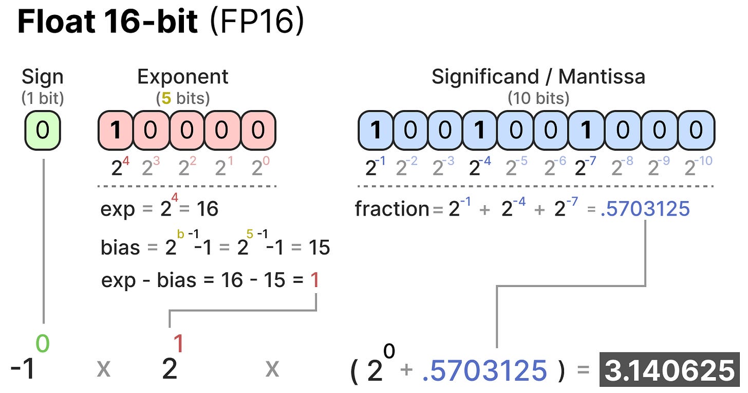
Formats such as FP16, FP32, FP64 use a sign / exponent / mantissa layout (“$1+e+m$ bits”):

S
E
M
sign
1 bit
exponent
$e$ bits
mantissa
$m$ bits

What does the bit string represent?

Normal numbers

Normal numbers ($E \neq 0$, not all-ones)

\[ \begin{gathered} V = (-1)^{s} \times 2^{n(E)-\mathrm{bias}} \times \bigl(1 + n(0.M)\bigr), \\[0.25em] \mathrm{bias} = 2^{e-1}-1. \end{gathered} \]

Here $n(E)$ is the integer encoded by the exponent field, and $n(0.M)$ is the fractional value of the mantissa bits.

Subnormals, zero, and specials

Subnormals and zero ($E = 0$)

\[ V = (-1)^{s} \times 2^{1-\mathrm{bias}} \times n(0.M). \]

Special numbers ($E$ all ones)

  • $M = 0$ $\rightarrow$ $\pm\infty$
  • $M \neq 0$ $\rightarrow$ NaN

FP16 encoding cases

FP16 bit layout and encoding cases

FP16 encoding cases (normals, subnormals, specials).

Common ML dtypes

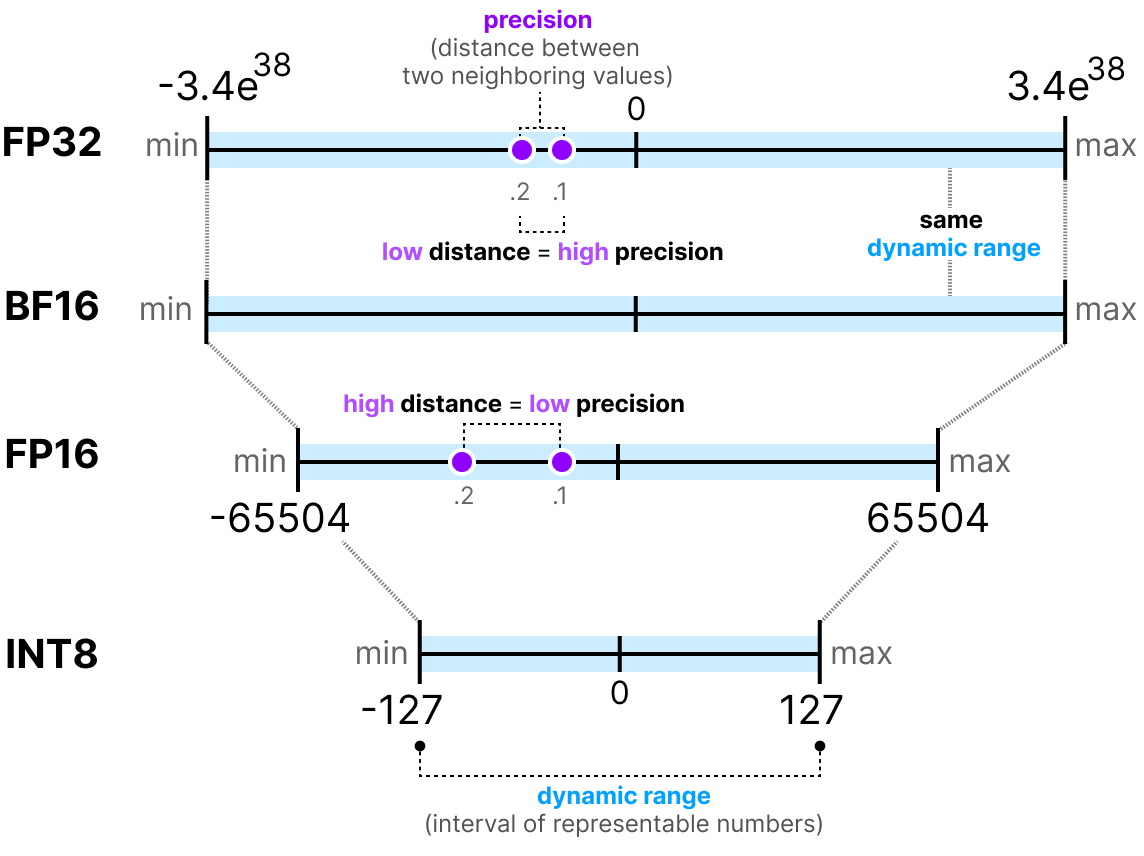
Precision and range of common dtypes

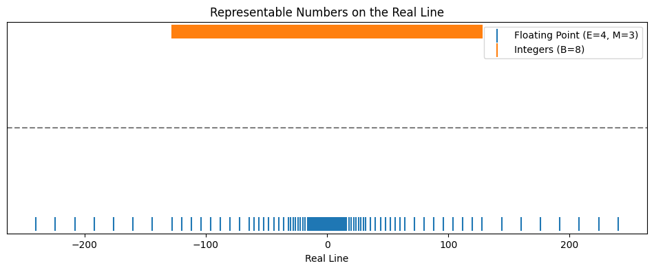
Common ML dtypes (FP32, BF16, FP16, INT8, …) trade precision (spacing between representable points) against range (max − min representable value).

Quantization in ML

FP32 and FP16 are the common “go-to” formats, but efficient ML often pushes further toward smaller bit widths:

\[ \mathrm{FP16,\ FP32} \;\longrightarrow\; \mathrm{FP8,\ INT8,\ INT4,\ \dots} \]
FP8 format overview

What we quantize

The objects we quantize are usually tensors or matrices: weights, activations, KV cache entries, and similar model states / optimizer states.

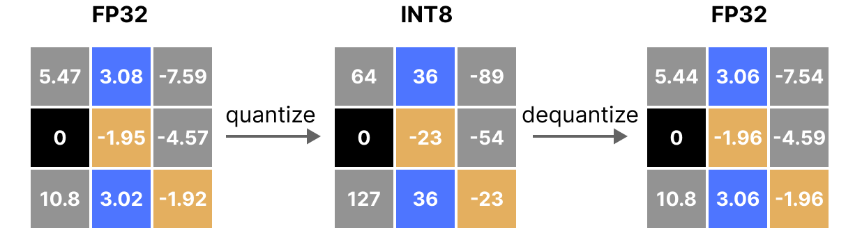
Example matrix of floating-point values

Dynamic vs. static quantization

  • Dynamic quantization. Treat the current matrix $M$ as the target data and fit $Q$ just for that tensor. If $M$ is an activation batch, the map must be recomputed when the data changes.
  • Static quantization. Treat $M$ as a sample from a target distribution; compute $Q$ once (e.g. from calibration data) and reuse it.

Either way, once we have a tensor or a calibration distribution, the core design question is how to place a small number of integer codes on the real line.

Designing $Q$

Q. Given a set of values, how do we design $Q$?

Example set of floating-point values

Target of quantization: signed $b$-bit integer codes: there are $2^b$ representable values, with range

\[ q \in \bigl\{-2^{b-1},\ldots,2^{b-1}-1\bigr\} \]

(e.g. $b=8$ gives $-128,\ldots,127$). How we place those levels on the real line really depends on the data.

Simplest function that can map $\{-2^{b-1},\ldots,2^{b-1}-1 \}$ to $[-r_{\max}, r_{\max}]$ is a linear function.

Linear and affine quantization

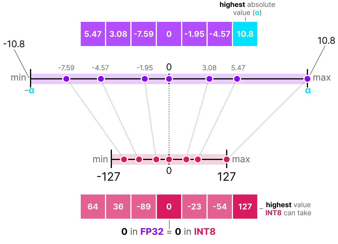
The simplest answer is to use a uniformly spaced grid. Symmetric linear quantization diagram

Linear quantization: real value $r$ is mapped to integer code $q$ using the scale $\lambda$: $r = \lambda q$.

Symmetric linear map

\[ Q(r) = \left[ \frac{r}{\lambda} \right]_Q \] \[ Q^{-1}(q) = \lambda q \]

Choose $\lambda$ so the largest magnitude maps to the largest positive code.

\[ r_{\max} = \max_i |x_i|,\quad q_{\max} = 2^{b-1}-1,\quad \lambda = \frac{r_{\max}}{q_{\max}}. \]
Why use $q_{\max}=2^{b-1}-1$? : For symmetry.

Why use linear quantization?

  • Simple, and only need to store one parameter: the scale $\lambda$.
  • Many elementary operations can be done in quantized space (especially useful for inner products, which are ubiquitous in ML)
    \[ Q(Q^{-1}(q_1) + Q^{-1}(q_2)) = q_1 + q_2 \]

When $r=\lambda q$ is inefficient

Q. When is a pure scale map bad?

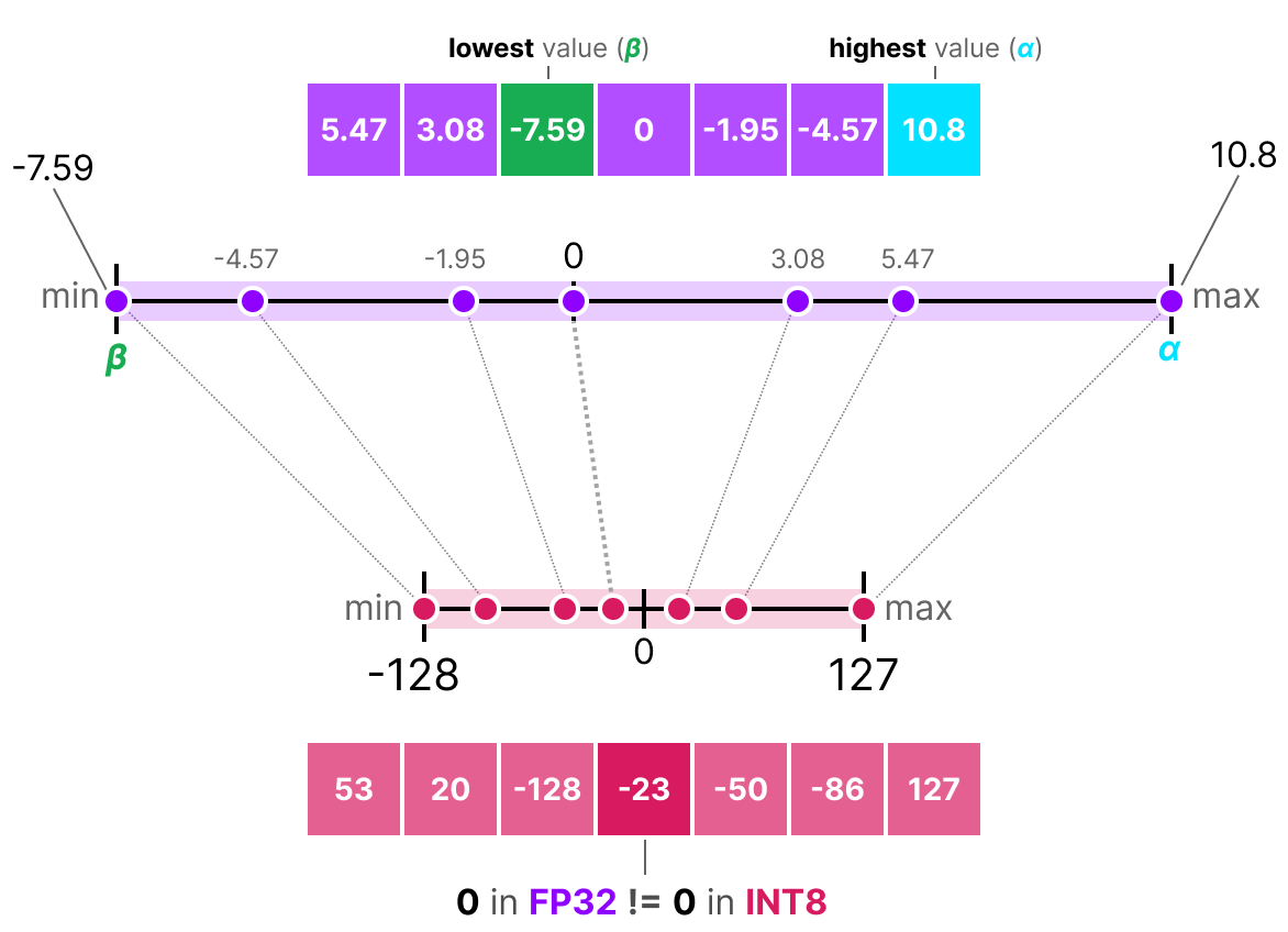
When the distribution is shifted / asymmetric: a zero-centered integer grid wastes codes on an empty region of the real line.

Symmetric linear quantization diagram

Affine (asymmetric) quantization

To move the grid left or right, introduce a zero-point $z_q$ as well as a scale:

Affine (asymmetric) quantization diagram
\[ r = \lambda(q - z_q). \]

Affine (asymmetric) quantization

  • Map data extremes to code endpoints:
    • $r_{\max} \mapsto q_{\max}$
    • $r_{\min} \mapsto q_{\min}$
    • $q_{\min} = -2^{b-1}$, $q_{\max} = 2^{b-1}-1$
  • Solve:
    \[ r_{\max}=\lambda(q_{\max}-z_q), \qquad r_{\min}=\lambda(q_{\min}-z_q) \]

Fitting $\lambda$ and $z_q$

\[ \lambda = \frac{r_{\max}-r_{\min}}{q_{\max}-q_{\min}}, \qquad z_q = q_{\max} - \frac{r_{\max}}{\lambda}. \]

Other failure modes?

Q. When can linear quantization still fail?

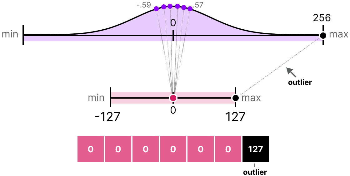
Outliers. A few extreme values stretch the scale, so most of the mass gets too few effective bits.

Outliers stretching the quantization range

Outliers consume dynamic range that the bulk of the data needs.

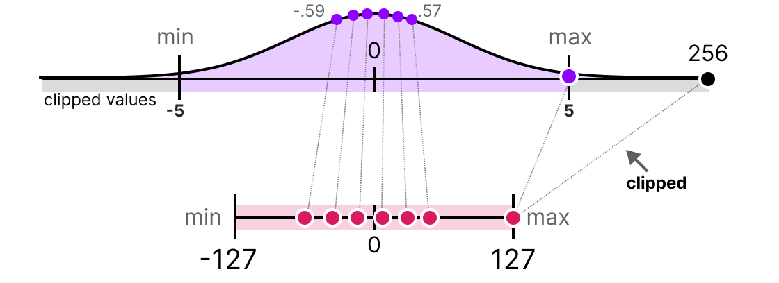
Clipping

Clipping outliers before quantization Effect of clipping on effective bit usage
  • Clip extreme values before fitting the quantization scale.
  • Useful if outliers are noise or unimportant. (example: gradient tensors)
  • Tradeoff: higher precision for typical values, but clipped values are distorted.

6. What if outliers are important?

absolute magnitude weight identifiers

E.g. Activation tensors are being quantised.

One approach: Separately store a sparse mask.

Rotate the vector

Alternatively "Rotate the Vector" to redistribute the energy

|·| x
\(\rightarrow\)
|·| Rx

Quantisation after rotation

\[ Q(\vec{x}) \rightarrow Q(R\vec{x}) \]
Quantisation of vector
Element wise quantisation.

* we can use linear quantisation for \(Q\).

How do we choose a rotation matrix

If \(\vec{x}\) was fixed / unknown?

  • e.g: [fixed] weight matrix
  • e.g: [unknown] Activation matrix

If \(\vec{x}\) was fixed

Say, \(\vec{x}\) was fixed.

A. Determine \(R\) which is optimal.

\(\Rightarrow\) But now you have to store \(R\) or \(R^{-1}\in\mathbb{R}^{d\times d}\)

\(R\): needs to be structured to reduce the memory footprint.

Can a fixed \(R\) be good?

A given structured matrix may or may not work for a specific \(\vec{x}\).

Side Note: In fact for any chosen \(R\), there is a \(\vec{x}\) for which \(R\vec{x}\) is catastrophic w.r.t quantisation!!

\(\rightarrow\) Example?

What should we do?

[Idea] Randomisation

Random and structured

Random

So that with high probability, \(Rx\) is not adversarial.

Structured

It can be stored efficiently.

Hadamard

Example of commonly used transforms

Randomised Hadamard

Let \(n=2^k\).

\[ H_2 = \begin{pmatrix} 1 & 1 \\ 1 & -1 \end{pmatrix} \]
\[ H_n = H_{2^k} = \begin{pmatrix} H_{2^{k-1}} & H_{2^{k-1}} \\ H_{2^{k-1}} & -H_{2^{k-1}} \end{pmatrix} \]
\[ \bar{H_n} = \frac{1}{\sqrt{n}}H_{n} \]

Randomized Hadamard

\[ R = \mathrm{Diag}(\vec{s})\cdot \bar{H_n} \]

\(\vec{s}\): Random sign vector

\[ s_i \sim \{\pm 1\} \quad\text{with equal probability.} \]

why hadamard

Computational Complexity of transforming nxn matrix

\[ O(n^3)\rightarrow O(n^2\log n) \]

Note that this is additional computation that we are introducing.

'HadaCore': Kernel for Hadamard transform. https://pytorch.org/blog/hadacore/

Memory Cost

1 sign bit per element.

* Note: we can avoid this \(O(n)\) memory by using Universal Hash functions. (More on that later)

Analysing effect of Hadamard on outliers

\[ R = \frac{1}{\sqrt{n}} Diag(\vec{s}) H_{n} \]
Given \(x\), let \[ y = Rx \]

A coordinate of \(y = Rx\)

Given \(x\), what is the probability that some coordinate of \(Rx\) is greater than \(M\).

\[ P(y_i \gt M) = ? \]

\(y=Rx\)

\[ y = Rx \]
\[ y_i = \sum_j r_{ij}\, x_j = \sum_j \frac{1}{\sqrt{n}} s_j h_{ij} x_j \] where $h_{ij} \in \{\pm 1\}$
\[ E(y_i) = ? \]
\[ E(y_i) = 0 \]
\[ \mathrm{Var}(y_i) = ? \]
\[ \mathrm{Var}(y_i) = \sum_j x_j^2 \frac {1}{n} \frac {1}{4} = \frac{1}{4} \|x\|_2^2 \]

Tail bound: Hoeffding

Which tail bound do we use?

Each term in \(y_i\) is bounded, so Hoeffding applies. Let \(X_1,\ldots,X_n\) be independent with \(X_j \in [a_j,b_j]\) almost surely, and \(S=\sum_j X_j\). For \(t>0\),

\[ \mathrm{Pr}\big(S - \mathbb{E}[S] \ge t\big) \le \exp\!\left( -\frac{2t^2}{\sum_j (b_j-a_j)^2} \right) \]
\[ \mathrm{Pr}\big(|S - \mathbb{E}[S]| \ge t\big) \le 2\exp\!\left( -\frac{2t^2}{\sum_j (b_j-a_j)^2} \right) \]

Exercise: Derive the Chernoff bound for the same sum.

Hoeffding applied to \(y_i\)

\[ y_i = \sum_j X_j, \qquad X_j = \frac{1}{\sqrt{n}} s_j h_{ij} x_j \]

Random signs \(s_j h_{ij}\in\{\pm 1\}\), so \(X_j \in [a_j,b_j]\) with

\[ a_j = -\frac{|x_j|}{\sqrt{n}}, \qquad b_j = \frac{|x_j|}{\sqrt{n}}, \qquad (b_j-a_j)^2 = \frac{4 x_j^2}{n} \]

\(\mathbb{E}[y_i]=0\). Plug \(t=M\) into two-sided Hoeffding:

\[ \mathrm{Pr}(|y_i| \gt M) \le 2\exp\!\left( -\frac{2M^2}{\sum_j (b_j-a_j)^2} \right) = 2\exp\!\left( -\frac{2M^2}{\sum_j 4 x_j^2 / n} \right) \]
\[ \mathrm{Pr}(|y_i| \gt M) \le 2\exp\!\left( -\frac{n M^2}{2\|x\|_2^2} \right) \]

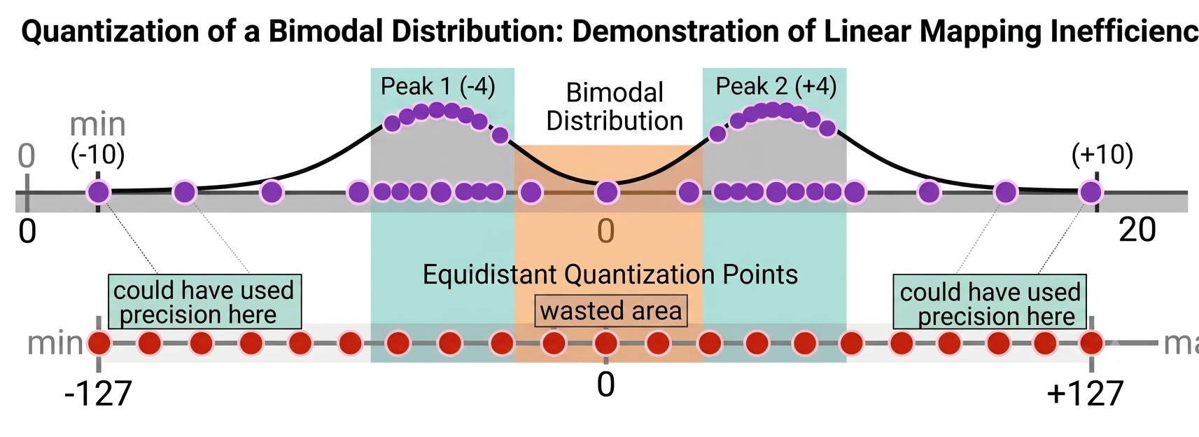
7. Another failure mode - multimodal distributions

Q. Where else does linear quantization fail?

Multimodal distributions. A uniform grid spends codes evenly across an interval, but the data may live in separated clusters with empty space between them.

Linear grid failing on a multimodal distribution

Linear levels miss multimodal structure.

Codebook / Clustering

  • Q. What can we do?
  • Idea: Learn a set of centroids $\{c_i\}$. (K-means, etc.)
  • Store each value as the index of its nearest centroid (codebook assignment).
  • Pros: Flexible, data-adaptive quantization that fits skewed or multimodal distributions.
  • Cons: Dequantization requires a table lookup; arithmetic needs dequantizing values first.
  • Tradeoff: Gains flexibility, loses some hardware simplicity of linear quantization.

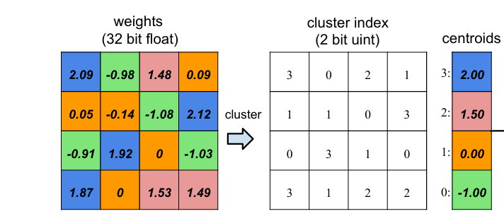
Weight clustering

Weight clustering into codebook indices and centroids

Weight clustering: float weights mapped to low-bit cluster indices plus centroids.

Linear vs. codebook

Aspect Linear quantization Codebook (non-linear)
Mapping Affine: $q=\mathrm{round}(x/s)+z$ Lookup: $q=\arg\min_i |x-c_i|$
Reconstruction $x\approx s(q-z)$ $x\approx c_q$
Best for Roughly uniform / unimodal mass Skewed or multimodal mass
Hardware Excellent (integer ops) Moderate / poor
Compute Often stays in quantized space Usually needs dequantization

8. Linear quantization: effect on inner products

Reconstruction error is only a proxy — quantized values are used in downstream computation. The simplest case: an inner product.

  • $w$ — quantized weights
  • $x$ — input / activation vector
  • $\Delta$ — quantization error on $w$
\[ \hat{w} = w + \Delta. \]

The quantized inner product

Q. What is $\langle \hat{w},\, x\rangle$, and how well does it approximate $\langle w,\, x\rangle$?

Deterministic rounding to nearest

Assume a grid of precision $\delta$ (spacing between representable values). Round-to-nearest guarantees

\[ |\Delta_i| \le \frac{\delta}{2} \qquad\text{for all } i. \]

The quantized inner product expands as

\[ \langle x,\, \hat{w}\rangle = \sum_i x_i\,(w_i + \Delta_i) = \langle x,\, w\rangle + \sum_i x_i\,\Delta_i. \]

Worst case (nearest)

If the signs align, every term $x_i\Delta_i$ can push in the same direction.

For example, take $x_i \ge 0$ and $\Delta_i=\delta/2$ for all $i$. Then

\[ \bigl|\langle x,\, \hat{w}\rangle - \langle x,\, w\rangle\bigr| = \frac{\delta}{2}\sum_i |x_i| = \frac{\delta}{2}\,\|x\|_1. \]

Squaring gives a worst-case squared error of order

\[ \mathrm{MSE}_{\text{nearest}}^{\text{(worst)}} = \frac{\delta^2}{4}\,\|x\|_1^2. \]

Round-to-nearest minimizes per-coordinate error, but the inner-product error can still accumulate coherently across coordinates.

Stochastic rounding

Suppose $w_i$ lies between consecutive grid points $a \lt w_i \lt b$ with $b-a=\delta$. Stochastic rounding sets

\[ \hat{w}_i = \begin{cases} a & \text{with probability } \dfrac{b - w_i}{b - a}, \\[0.6em] b & \text{with probability } \dfrac{w_i - a}{b - a}. \end{cases} \]

Equivalently, $\hat{w}=w+\Delta$ with a random per-coordinate error $\Delta_i$.

Unbiasedness

\[ \mathbb{E}[\Delta_i] = 0 \quad\Rightarrow\quad \mathbb{E}[\hat{w}] = w. \]
\[ \langle x,\, \hat{w}\rangle = \langle x,\, w\rangle + \sum_i x_i\,\Delta_i, \]
\[ \mathbb{E}\!\bigl[\langle x,\, \hat{w}\rangle\bigr] = \langle x,\, w\rangle. \]

The quantized inner product is unbiased.

Variance / MSE

Assuming independent rounding noise across coordinates,

\[ \mathrm{Var}\!\bigl(\langle x,\, \hat{w}\rangle\bigr) = \sum_i x_i^2\,\mathrm{Var}(\Delta_i). \]

With fractional part $\alpha_i=(w_i-a)/\delta \in [0,1]$,

\[ \mathrm{Var}(\Delta_i) = \alpha_i(1-\alpha_i)\,\delta^2 \le \frac{\delta^2}{4}. \]

Therefore

\[ \mathrm{MSE}_{\text{stochastic}} = \mathrm{Var}\!\bigl(\langle x,\, \hat{w}\rangle\bigr) \le \frac{\delta^2}{4}\sum_i x_i^2 = \frac{\delta^2}{4}\,\|x\|_2^2. \]

The bound can be smaller still, depending on the actual fractional parts $\{\alpha_i\}$ and on $x$.

Nearest vs. stochastic

\[ \underbrace{\frac{\delta^2}{4}\,\|x\|_1^2}_ {\text{worst-case nearest}} \qquad\text{vs.}\qquad \underbrace{\frac{\delta^2}{4}\,\|x\|_2^2}_ {\text{MSE stochastic}}. \]

Since $\|x\|_2 \le \|x\|_1 \le \sqrt{d}\,\|x\|_2$, the $\ell_1$ worst case can be up to a factor $d$ larger in squared error than the stochastic $\ell_2$ MSE, especially for dense $x$.

Takeaway Round-to-nearest is optimal per coordinate, but for the inner product the errors can add coherently. Stochastic rounding keeps the estimate unbiased and replaces an $\ell_1$-scale worst case with an $\ell_2$-scale MSE.

9. Granularity of Quantization

To define a quantization scheme, we need to decide which weights to group together for quantization. This choice determines the granularity of quantization.

  • Entire model: Apply the same quantization parameters (e.g., scale and zero point) to all weights in the model.
  • Entire layer: Quantize all weights within a layer together.
  • Attention heads: Apply separate quantization to each attention head.
  • Single tensor: Quantize individual tensors (matrices or vectors) separately.
  • Parts of a tensor: Further divide tensors (e.g., by rows, channels, or blocks) and quantize the pieces independently.

Finer granularity (quantizing smaller groups separately) can improve accuracy by adapting quantization to the distribution of each group, but may require storing more quantization parameters.

Hardware supported quantization