Efficient AI
Pruning / Sparsity
Aditya Desai
Many thanks to all the resources listed in References on the main website. Almost all figures are taken from these resources; some were generated with Gemini. Some images are taken from Google Images and still need proper citation (in progress).
Size of AI is huge and it is only growing!
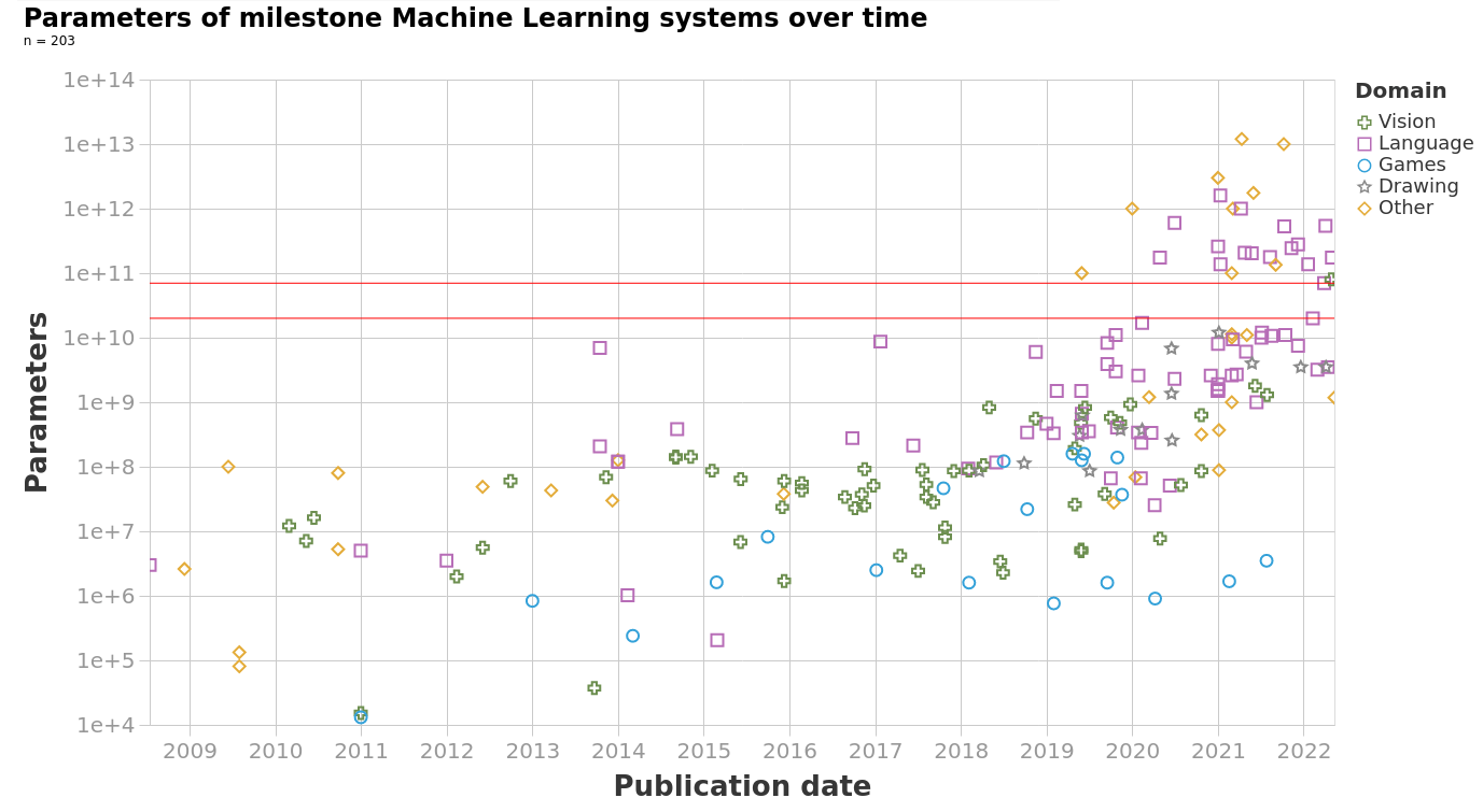
Deployment targets have tight memory budgets
| Device Class | Approximate RAM Range |
|---|---|
| Tiny IoT devices | KB to MB |
| Wearables | 0.5–8 GB |
| Phones & Glasses | 4–16 GB |
| Laptops | 8–64 GB |
| Drones | 2–32 GB |
| Cars | 16–512 GB |
| Edge Servers | 64 GB–4 TB |
Energy cost of compute vs memory
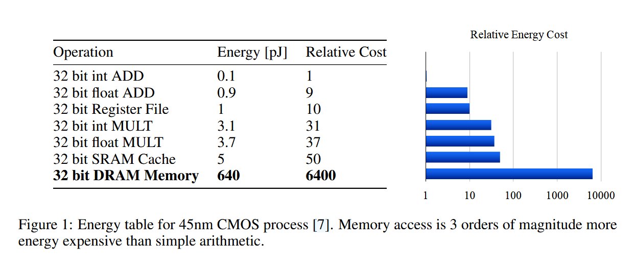
- Memory access (DRAM) is ~3 orders of magnitude more energy-expensive than simple arithmetic.
- Compressing models reduces data movement as well as FLOPs — often the bigger win for energy.
what is model compression?
- Given a trained model, can we reduce its size and computation while maintaining its accuracy?
why model compression?
- saves memory, compute, energy, money, etc
- Unlocks new deployment scenarios. e.g. deploying on edge devices -- PCs/laptops/phones/cars/drones/etc
Techniques are transferrable..
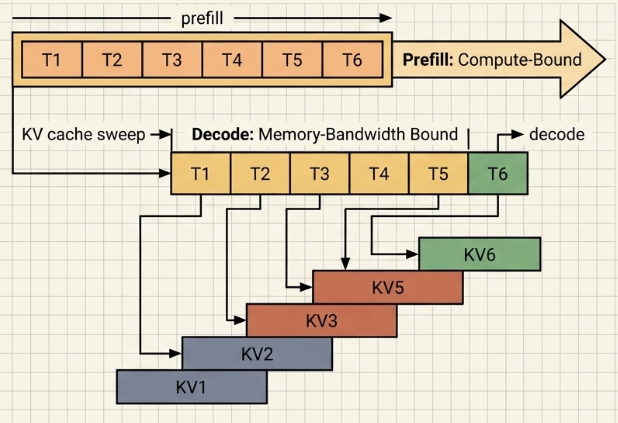
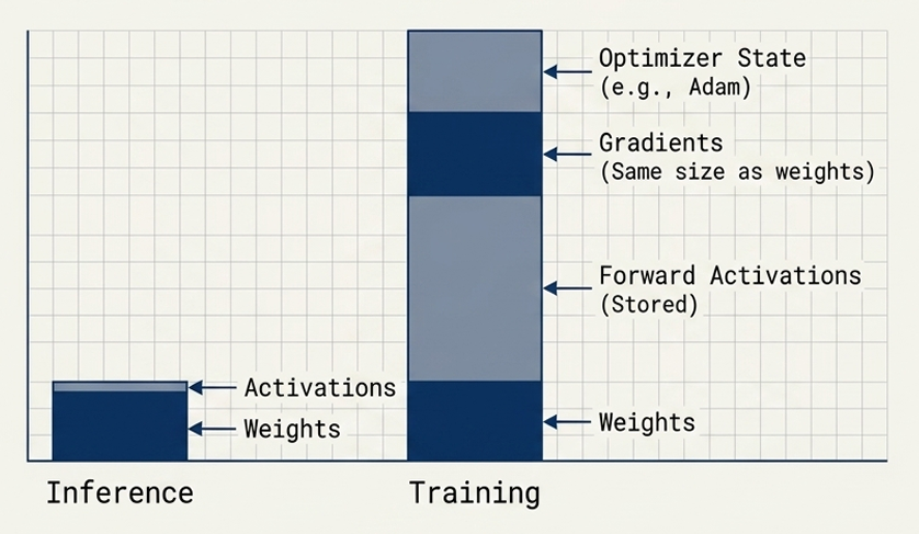
We can apply the techniques we will discuss as part of model compression to activations, gradients, optimizer states, etc.
Techniques are transferrable..
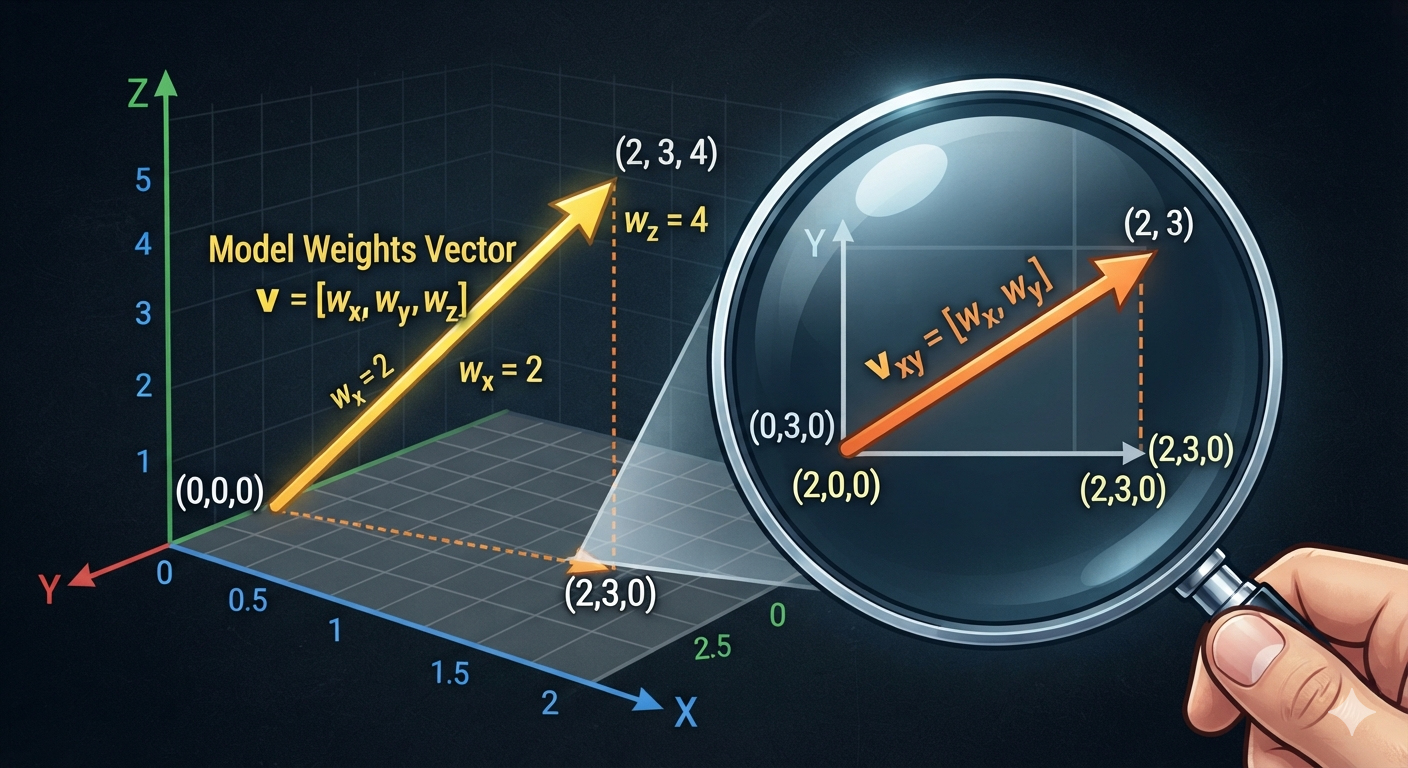
- Pruning is just one structured lens.
- We can think of other forms of low-dimensional spaces or quantizations of space.
- The spaces onto which we project are different, but the principles are the same.
Pruning / Sparsity
- what is pruning?
- Pruning a neuron
- Optimal Brain Surgeon
- Optimal Brain Compression
- Iterative Magnitude Pruning
- Pruning in Pre-LLM era
- Structured Pruning & Hardware Supported Sparsity
- Sensitivity Analysis for Pruning
- Lottery Ticket Hypothesis? (If we have time)
- Pruning LLMs
Two useful identities for inverse of a matrix
1) Rank-one update — add outer product $uv^\top$ to $A$:
If you do a one-rank update to A, then it provides a relation between inverse
of A and the inverse of the updated matrix.
O(n2) update instead of O(n3) for inverse of (A+uv^\top)
Inverse of a submatrix extraction
\[ A = \begin{pmatrix} a_{11} & a_{12} & a_{13} \\ a_{21} & {\color{#0b6e4f}a_{22}} & {\color{#0b6e4f}a_{23}} \\ a_{31} & {\color{#0b6e4f}a_{32}} & {\color{#0b6e4f}a_{33}} \end{pmatrix} \;\longrightarrow\; B = A[2{:},2{:}] = \begin{pmatrix} {\color{#0b6e4f}a_{22}} & {\color{#0b6e4f}a_{23}} \\ {\color{#0b6e4f}a_{32}} & {\color{#0b6e4f}a_{33}} \end{pmatrix} \] Relation between $A^{-1}$ and $B^{-1}$
If you have inverse of a larger matrix, then you can use this to find the inverse of matrix
with one row and column removed.
O(n2) update instead of O(n3) for inverse of B
Pruning: Sparsity in weights
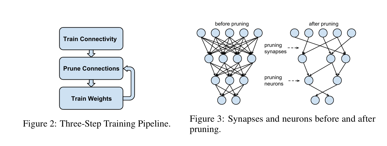
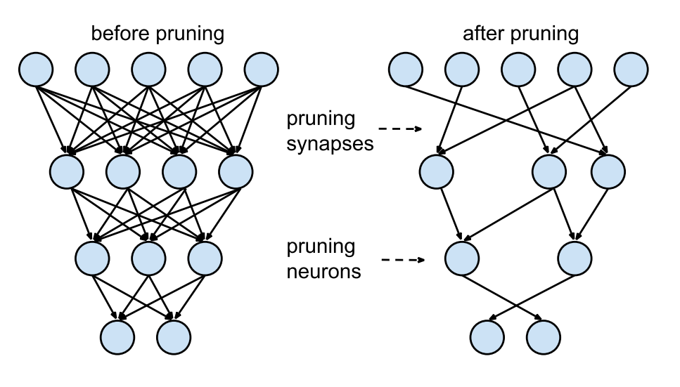 Computational graph view: we remove some of the connections in the model.
- Removing enough connections can naturally remove some of the neurons and structural components in the model.
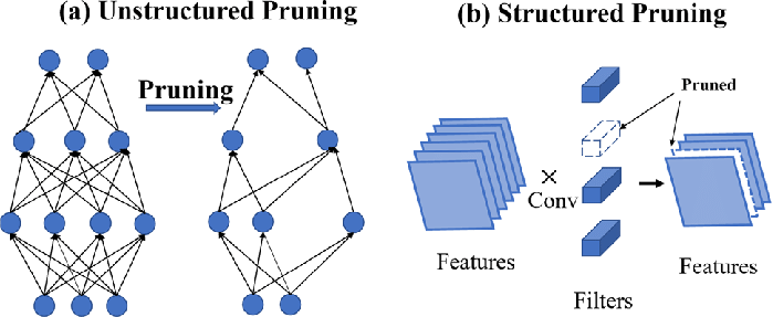
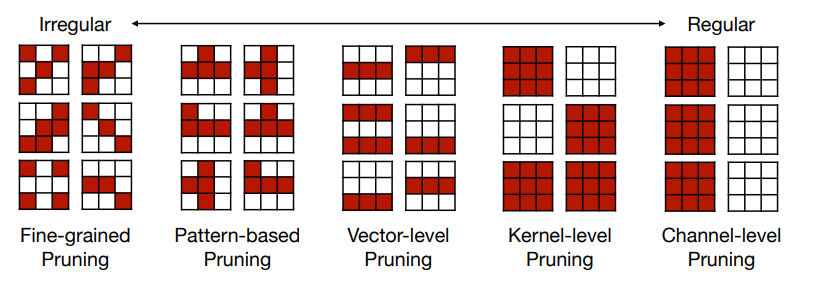
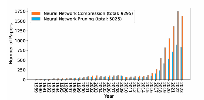
Pruning
- Pruning has a history since 1980s and post deep learning era it is one of the most widely researched techniques
Pruning a neuron
Note Link: notes/pruning_a_neuron.html
what is the complexity of this computation
x, w \in R^d, y \in R- Single neuron pruning:
-
d×O(d3)d— number of sub problemsO(d3)— inverse of the Hessian
If pruning k neurons, then the complexity is
O(k d4)
A single neuron pruning
- Pruning a neuron itself is quite expensive (disclaimer: this is not the best algo)
- Imagine decent sized model pre-LLM (Convolution / MLP etc)
- Imagine a LLM model!
Pruning a “Model"
(Optimal Brain Surgeon(OBS), Hassibi and Stork, 1993)
Note Link: notes/pruning_a_model.html
All that one needs to know for pruning.
Algorithm for OBS
- Train a “reasonably large” network to minimum error.
- Compute
H−1. -
Find the
qthat gives the smallest saliencyLq = wq2 / (2 [H−1]qq). If this candidate error increase is much smaller thanE, delete theq-th weight and go to step 4; otherwise go to step 5. -
Use the
qfrom step 3 to update all weights (δw). Go to step 2. -
No more weights can be deleted without a large increase in
E. (At this point it may be desirable to retrain the network.)
Complexity of OBS?
- A single step: Dominated by forming / inverting the Hessian:
O(N3), whereNis the number of parameters. - Hessian computation is
O(nN2)wherenis the number of samples andNis the number of parameters. - k step OBS :
O(k(N3 + nN2))
How can we reduce the complexity of OBS?
Hint: Use Linear Algebra identities we introduced. (Exercise : We will look at it next class)
How can we simplify
\[ Saliency(q) = L_q = \frac{w_q^2}{2 H^{-1}_{qq}} \] \[ Update(w) = \frac{w_i}{H^{-1}_{qq}} H^{-1} e_i \]Optimal Brain Damage (OBD)?
assumptions- The model is trained to convergence.
- The model is a quadratic local approximation.
- Hessian is a diagonal matrix.
Algorithm for OBD
- Train a “reasonably large” network to minimum error.
- Compute Hessian H
-
Find the
qthat gives the smallest saliencyLq = ½ Hqq wq2.Delete few low saliency weights -
Update all weights (δw). - Retrain i.e. go to step 1.
Complexity of OBD?
- We only need diagonal entries of Hessian.
Computing diagonal entries of Hessian
Hint: Can be done in single forward / backward pass. (Exercise : We will look at it next class)
- The hessian diagonal computation is of the same order as the gradient computation.
Further simplifications: Iterative Magnitude Pruning (IMP)
- Completely let go of the data consideration
- Just prune the weights based on their
magnitude(equivalent to assumingH_{kk}is same for allk) and rely on training to correct the errors
Algorithm for IMP
- Train a dense network to convergence.
-
Compute the magnitude of each weight:
|wi|. - Remove weights with the smallest magnitudes (prune a fixed fraction or all below a threshold).
- Retrain the pruned network. Return to step 2 (iterate until target sparsity).
Iterative Magnitude Pruning (IMP)
- Simple and easy to implement
- Training is strictly required.
OBS vs OBD vs IMP (w/o re-training)
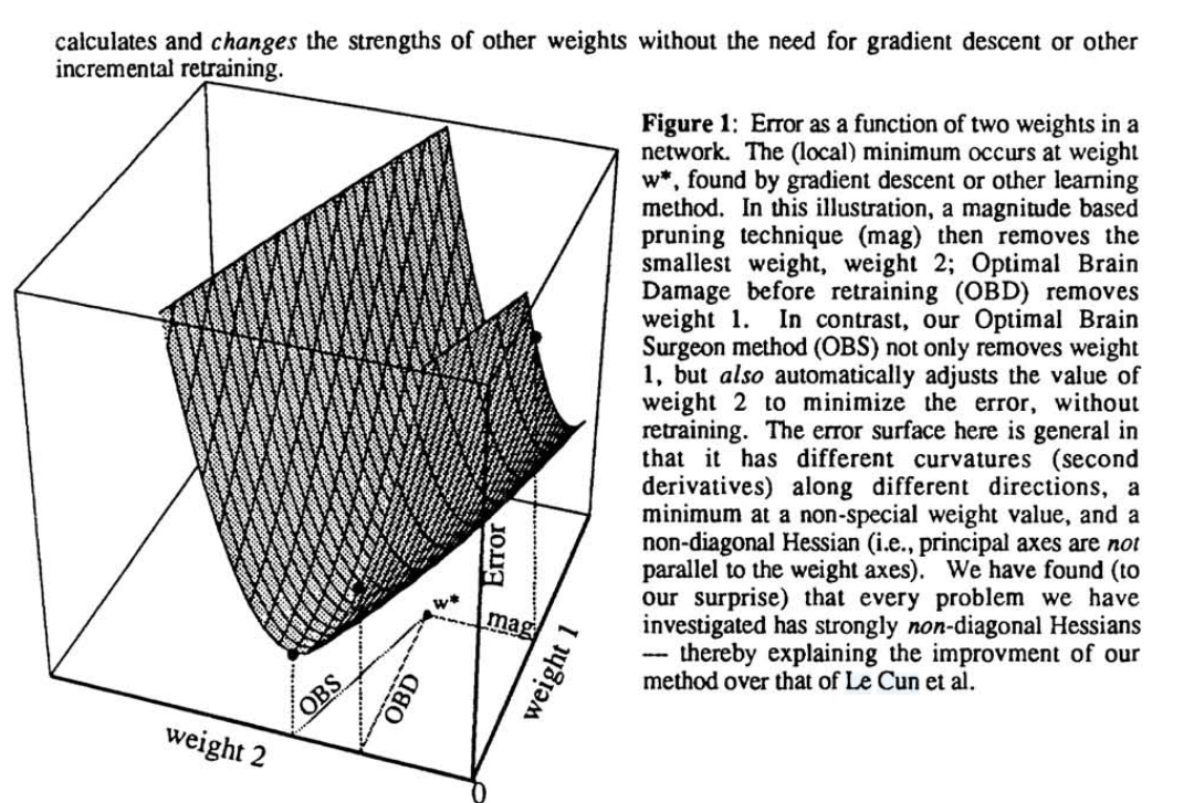
- OBD and IMP may lead to different pruning
- Implications of using "less" informed pruning methods can be significant when not re-trained.
General Framework for Pruning
- Train a dense network to convergence.
- Compute the saliency score of each weight
- Remove weights with the smallest saliency scores
- Retrain the pruned network. Return to step 2 (iterate until target sparsity).
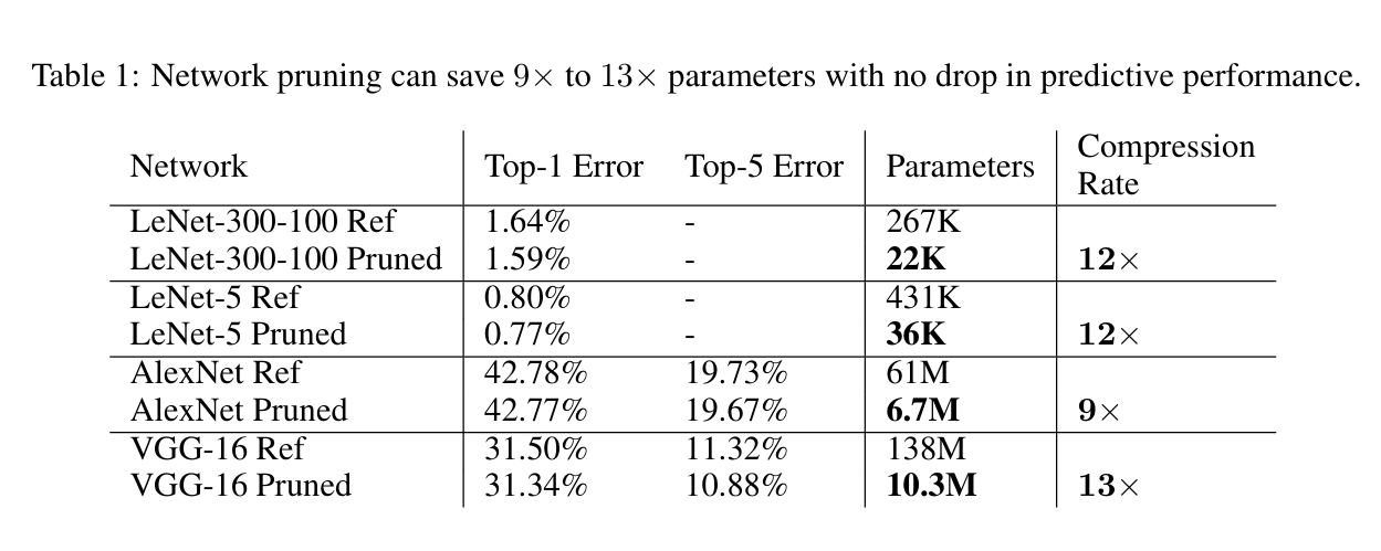
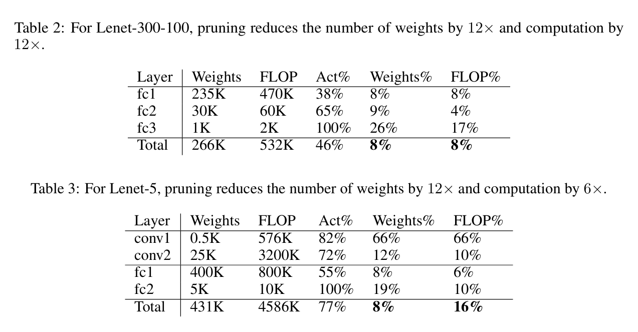
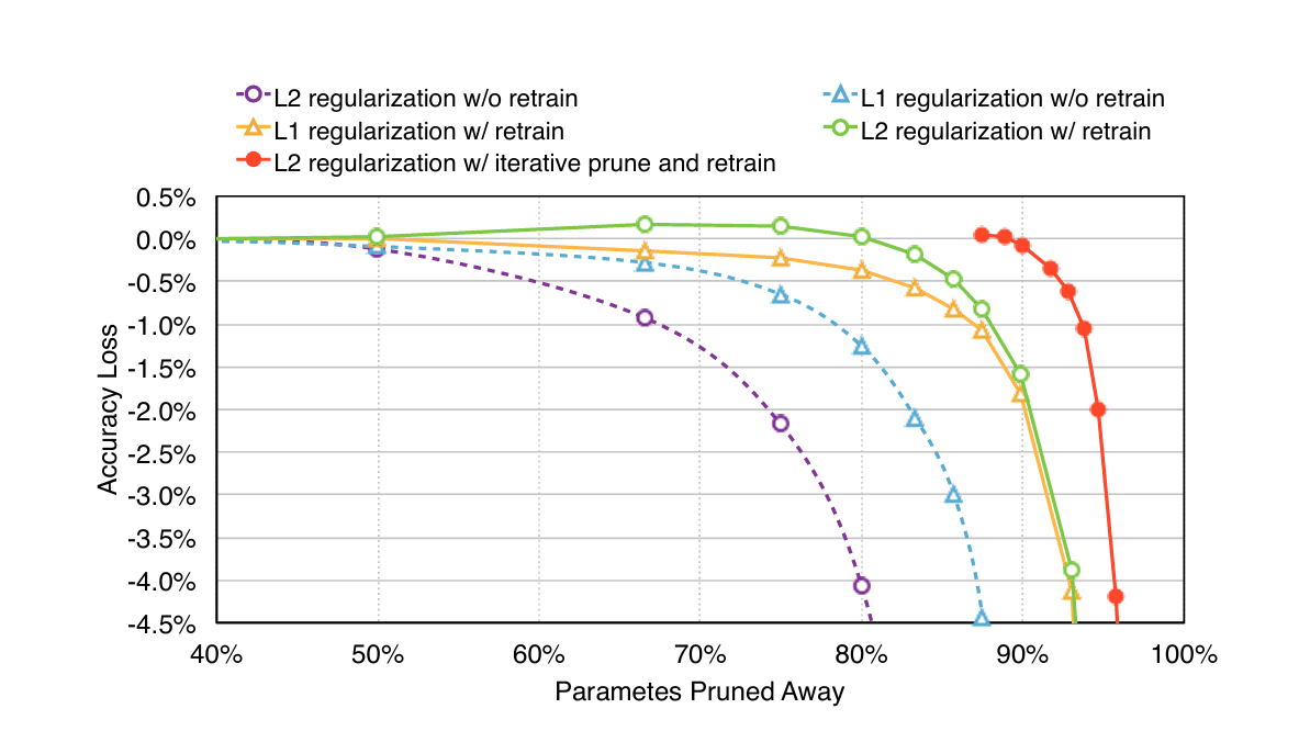
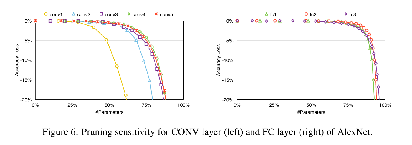
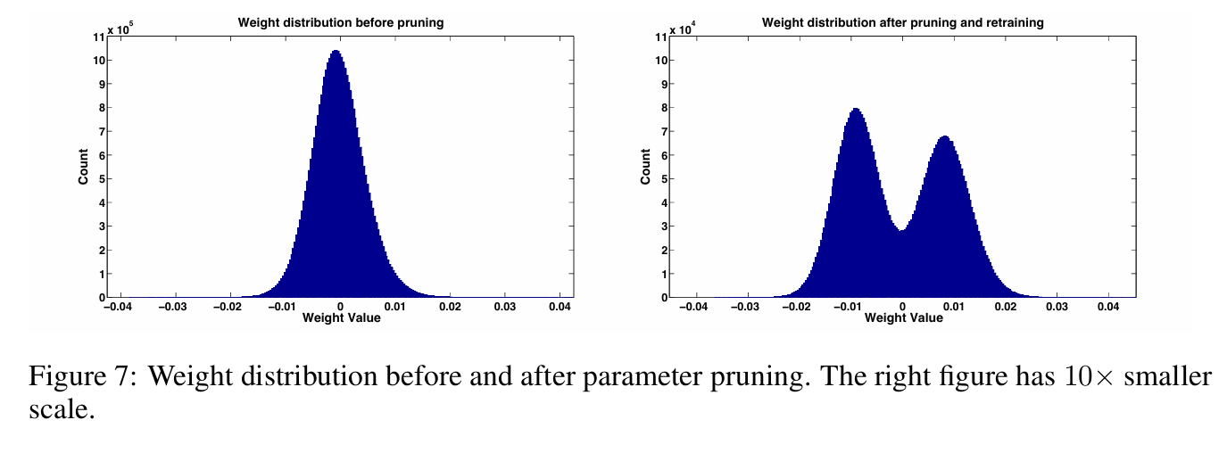
Results from the paper
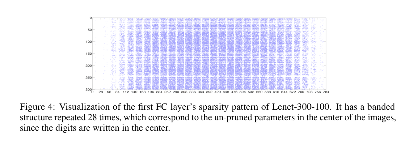
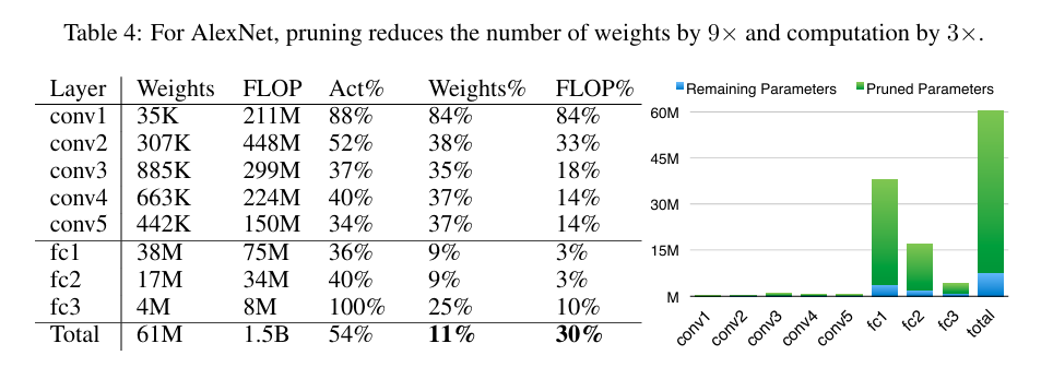
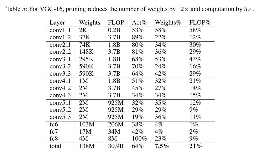
Learning both Weights and Connections for Efficient Neural Networks" by Han et al. 2015